
 Prioritizing one part over others is an easy way to speed up the production of the prioritized part. However, if too many parts are prioritized, the performance of the others will suffer.
My general recommendation is to prioritize no more than 30% of your production volume. In this post I will look in more detail at this relation and verify this assumption (TL;DR: this is correct!). This post is based on a masters thesis by my student Yannic Jäger.
Introduction
 Imagine you are waiting at a supermarket checkout. Based on the number of people in front of you, you can make a reasonable guess on when it will be your turn. However, if another customer would have a gold member VIP card, he could cut in line and be the next person that is served. If there is only one VIP member cutting in in front of you, your initial estimate would still be reasonably good. However, the more VIP members there are, the longer the poor and unimportant Non-VIP customer have to wait. In this post I will show you these relations in more detail.
In my previous blog posts I have written extensively on how to prioritize, and how NOT to prioritize, production (or other) systems. Back then I recommended not prioritizing more than 20%–30% of the parts. The detailed data below will confirm this estimate.
- How to Prioritize Your Work Orders – Basics
- How to Prioritize Your Work Orders – The VIP Lane
- How to Prioritize Your Work Orders – Prioritization of Made to Stock
- How to Prioritize Your Work Orders – Prioritization of Made to Order
Simulated System
To simulate the system, we used a simple one-process system. By adjusting the random arrival time and the random service time, we tested different utilizations between 75% (low utilization) to 95% (very busy system). We did not test 100%, because this would cause an infinite queue. The system processed two types of parts, simply called A and B. Both parts had the same randomly distributed processing time. For simplicity’s sake, we had a lot size of one and no set up times, breakdowns, or other disturbances.
Our system was set up for an exponentially distributed inter-arrival time with an average inter-arrival time of 6 minutes, or an arrival takt of 10 pieces per hour.
The processing rate is log-normal distributed, varied, with simulated values of 13.33; 12.50; 11.76; 11.11; and 10.35, giving an utilization 0f 75%; 80%, 85%, 90%, and 95% respectively. The standard deviation of the log-normal distribution was set up so that the coefficient of variation (standard deviation divided by the mean) was always 25%.
First-Come-First-Served Base System
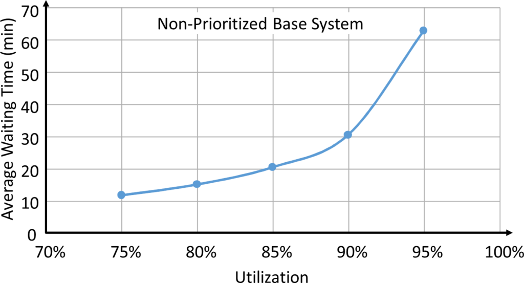
 As a baseline, we simulated the system with only one part, and with two parts without any prioritization. All parts were processed on a first-come-first-served basis. It makes no difference if you have only one part or if you have two parts without any prioritization, the system behaves identical. The only factors influencing the average waiting time are the relation between the total arrival rate and the total departure rate, which create different utilizations.
The average waiting time is shown below. As expected, it is an exponential relation. The higher the utilization, the longer the average waiting time. The average waiting time would go to infinity at 100% utilization (see also the Kingman formula here). It makes no difference if there is only one part type or two different part types, or if the percentage is A or B, as long as there is no prioritization and the total average arrival rate is 10 parts per hour.
Prioritized System
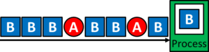
 Of course, we want to know the effect of prioritization. Hence, we now prioritize our parts. Parts of type A and B are waiting in separate queues. If there is one or more part A waiting, it always takes priority over any part B. Within the A queue and the B queue, we maintain FIFO respectively, although this would not influence our results.
We varied the percentage A using values of 0.1%; 10%; 20%; 30%; 40%; 50%; 60%; 70%; 80%; 90%; and 99.9%, spanning pretty much the entire range between almost no part A, and almost only part A.
Resulting Waiting Time
Below are the results for different percentages of prioritized parts A and different utilizations. You can also see the baseline of a non-prioritized system of similar utilization and overall arrivals and departures. This baseline would also be the weighted average of the average waiting time of A and B together.

The baseline always goes through the waiting time of 0.01% A parts (i.e., 99.9% B parts) and 99.9% A parts, as these are effectively only-B and only-A parts, and should behave like the unprioritized system.
Looking at the graphs above, you can see that having a few prioritized A parts will be beneficial for the A parts, without much drawback for the B parts. For example, up to 30% A parts, the A parts will pass through the system much faster, but slowing down the B parts only marginally.
However, as you increase the percentage of prioritized parts, the benefit will be less and less, until there is no longer any benefit to the A parts. But at the same time, there is a huge disadvantage and punishment for the B parts. If you prioritize, for example, 90% of the A parts, they behave very similar to the baseline system. However, the B parts are punished harshly.
Resulting Percentage Improvement over Unprioritized System
The effects can be seen very clearly in the graphs below, shown for different utilizations. The waiting time of the prioritized part A can be reduced to 13%–50% of the original system depending on the utilization. However, as you prioritize more parts, the effect becomes less and less, although even 70% prioritized A parts is still a significant improvement over the average.

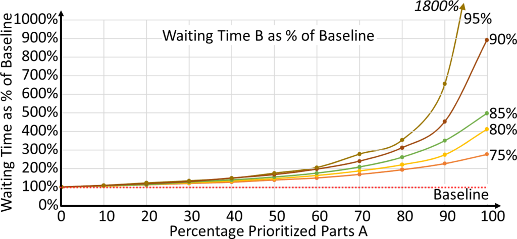
The real kicker and the reason why I recommend not prioritizing more than 30% of your parts is the behavior of the B parts. This is shown below for different utilizations. If only a few A parts are prioritized, the waiting time of the B parts is increased only slightly. For example, with 30% A parts prioritized, the waiting time of B increases 20%–30%. Not ideal, but manageable.
However, the waiting time increases exponentially. With 60% prioritized A parts, the waiting time of B doubles. For even more prioritized A parts, the waiting time increases to 300%–1800%, which is very likely to dissatisfy a customer waiting for parts.
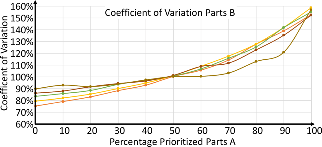
Coefficient of Variation of the Waiting Time
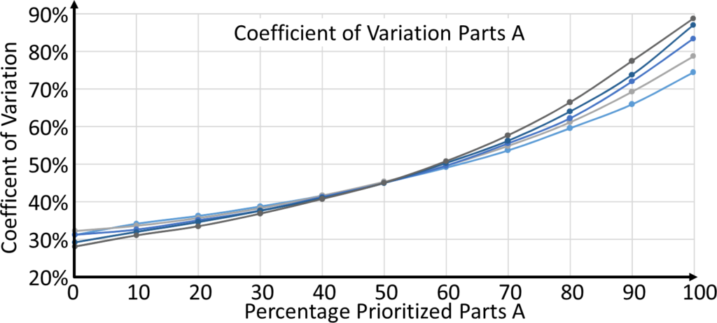
Another aspect worth looking at is the coefficient of variation in the waiting time (calculated as the standard deviation of the waiting time divided by the mean waiting time). These coefficients of variations are shown below for parts A and B depending for different prioritizations. The graph also shows the different utilizations as different lines, although these have little influence here.
Interesting is that with increasing prioritization, the coefficient of variation goes up. This means that the standard deviation is increasing more than the mean! From the point of view of the production planner, this is a very bad thing. A good production planner can handle longer lead times by including this in his planning schedule. However, if the standard deviation increases faster than the mean, it becomes more difficult to plan. The parts may be finished much earlier than planned, or much later than planned.
This means that being prepared for a frequent excessive delay over the average, you need to put the material in stock (if it is made-to-stock), or promise a much later delivery time (if it is made-to-order), or otherwise apologize profusely to the customer and feel the wrath of your boss because the delivery performance suffers (for both MTO and MTS)
In sum, not only does your waiting time increase, but the fluctuations increase even more, resulting in stock increases, late deliveries, low delivery performance, and unhappy bosses and customers.
Lesson Learned

Overall, it remains important to not prioritize too many parts. While the intent of accelerating the important parts is understandable, the benefit decreases with increasing prioritization. At the same time, the “unimportant” parts get more and more punished, and their waiting time increases exponentially. At one point these “unimportant” parts will become important again due to their very long lead times. Now, everything is important (and your boss doesn’t want to hear that this also means that nothing is really important). The production planner feels like he is getting an endless stream of hot potatoes that are needed right away, while the system does not have the capacity. At the same time, the planability goes down as the fluctuations increase!
Therefore, folks, please do not prioritize more than 30% of your production! This maintains a benefit for the prioritized parts, without damaging the not-so-important parts, while keeping fluctuations manageable (or at least not much worse than the initial system. Now, go out, prioritize smartly, and organize your industry!
Source
Jäger, Yannic. 2017. “Einfluss von Priorisierung auf das Verhalten eines Produktionssystems.” Master Thesis, Karlsruhe, Germany: Karlsruhe University of Applied Sciences.
Hi Christoph,
1. if there are present also change over time (lets assume Min 10x takt time=1h) the reasonable prioritization would be instead of 30% how much?
2. Or even add on to point 1.: 5 or more different products instead of only 2 (A and B)?
Thanks for your estimation.
Hi Matjaz, the products A and B represent two product groups, prioritized and not prioritized. It does not help to grade the products into 5 different priority levels (see How to Prioritize Your Work Orders – The VIP Lane). The prioritization is independent of change over times, although a change over sequence may also influence the prioritization (i.e. polymer light to dark sequence would have to be combined with the priority).