Determining the Size of Your FiFo Lane – The FiFo Formula

FiFo lanes are an important tool to establish a pull system. They are often combined with kanban. However, while there is a lot of information on how to calculate the number of kanban (the Kanban Formula), there is very little information available on how large a FiFo should be. In my last post I talked about why we need FiFo lanes. In this post I want to discuss how large a FiFo should be. The first part is a lot of mathematical theory, but you can easily skip ahead to the practical advice. In another post I have programmed a small FIFO calculator that does exactly these calculations.

The Mathematically Correct (and Practically Completely Useless) Solution

[Note: I have programmed a small tool that does the math for you: The FiFo Calculator – Determining the Size of your Buffers]

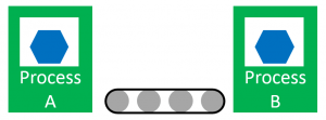
First, I would like to show you the mathematically rigorous approach – which turns out to be completely useless in practice. (For a practical approach, see below ). The mathematical approach uses probability functions. Assume you have two processes, A and B, that are randomly distributed as shown below.

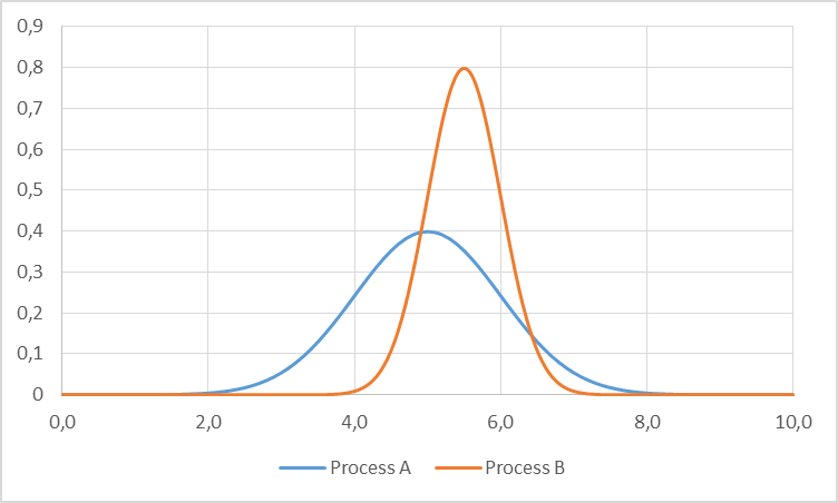
Below are two example probability distributions for these processes. These are standard normal distributions. These are, in fact, not good assumptions for processing times, since they start at minus infinity and hence can have negative values too. Nevertheless, these functions are probably the best known and are also illustrative, hence I use them here.

This can also be expressed mathematically as two probability density functions, given here for normal distributions:

\[ { f_A(x)=f(x,\mu_A,\sigma_A)=\frac{1}{\sigma_A \sqrt{2\pi}}e^{-\frac{(x-\mu_A)^2}{2\sigma^2_A}} }\]
\[ { f_B(x)=f(x,\mu_B,\sigma_B)=\frac{1}{\sigma_B \sqrt{2\pi}}e^{-\frac{(x-\mu_B)^2}{2\sigma^2_B}} }\]

The first process, A, has a mean of 5 and a standard deviation of 1. The second process is a bit slower with a mean of 5.5, but has a tighter standard deviation of 0.5. This means that in average process, B is the bottleneck with a mean cycle time of 5.5. However, sometimes by chance process A will be slower than process B and may become a temporary bottleneck.

Inventory (as, for example, a FiFo) tries to prevent the slow down of process B. The more inventory you have, the less likely it is that process B will be slowed down by process A. This will increase the overall system output. Please note that no matter what you do with your inventory, the system cannot become faster than process B.

 The “Simple” Case – No Inventory

In the most simple case, we have no inventory between two processes. In this case, the likelihood of the slower process B being temporarily slowed down by process A. Mathematically speaking, this is the probability of process A being slower than process B. This can be calculated by integrating as shown in the formula below, which gives us the probability of process A being slower than process B:

\[ {P(A>B)=\int\limits_{-\infty}^{+\infty}{f_A(x)\cdot \left( \int\limits_{-\infty}^x{f_B(x)dx} \right) dx} }\]

As any sum or difference of independent random variables will in almost all cases result in a normal distribution, the above can be also expressed as a normal distribution, where the mean and standard deviation can be calculated quite easily:

\[{ \mu_{A-B}=\mu_A-\mu_B }\]
\[ { \sigma_{A-B}=\sqrt{\sigma_A^2+\sigma_B^2} }\]

This can be visualized as in the  graph below. We see again our two initial distributions as above. The third gray curve is the distribution of the difference A–B. The likelihood of process A being faster than process B is the likelihood of the difference being larger than zero, represented by the shaded area.

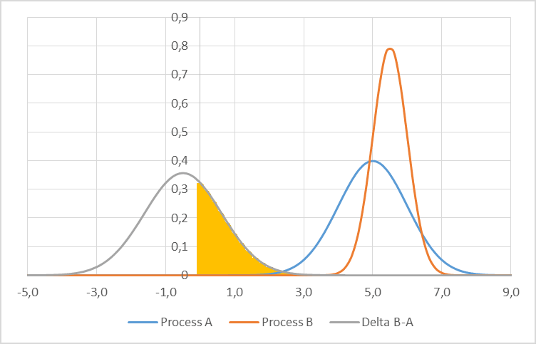
In our example with a mean of 5 and 5.5 and a standard deviation of 1 and 0.5 for process A and B respectively, this gives us a likelihood of process A being slower of 32.7%. In about 1/3rd of the cases, process B is slowed down by process A even though process B is on average the slowest process. Of course, this means that our system slows down. Instead of the maximum possible part every 5.5 time units, it is now a part every 5.75 time units. This gets worse with increasing standard deviations too.

Including Buffer to Increase Speed

Adding buffer between the processes reduces the likelihood of the normally faster process A slowing down the normal bottleneck process B. This means that the sum of two random times from process A has to be larger than the sum of two random times of process B. The distribution can be calculated as follows:

\[ {f_{2\cdot A}(z)=\int\limits_{-\infty}^{+\infty}{f_A(z-x)\cdot f_A(x)dx} }\]

Luckily, this too can be simplified to calculate the mean and standard deviation of a normal distribution as shown below:

\[ { \mu_{2\cdot A}=2\cdot \mu_A }\]
\[ { \sigma_{2\cdot A}=\sqrt{2\cdot\sigma_A^2} =\sqrt{2}\cdot\sigma_A }\]

Even more general, this can be calculated for the sum of any number of random times:

\[ { \mu_{n\cdot A}=n\cdot \mu_A }\]
\[ { \sigma_{n\cdot A}=\sqrt{n\cdot\sigma_A^2} =\sqrt{n}\cdot\sigma_A }\]

The means of these sum go up linear with the number of times included. The standard deviation, however, increases only with the square root of the number of times! Hence, while the relative distance between the sums for the process times stays equal, the with of the distribution becomes smaller.

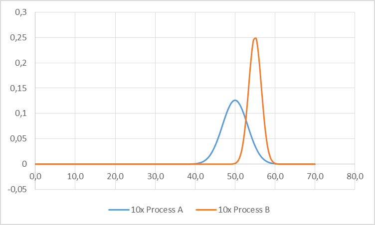
Below are the distributions for the sum of ten times process A and ten times process B. In comparison with the images above, the relative distance between the means did not change much. Process B is still 10% slower than process A. The width, however, has significantly decreased. For example, process A has a standard deviation of 1 for a cycle time of 5. Multiplying by 10 increases the sum of the cycle times to 50, but the standard deviation only to 3.16.

Relation between Buffer Size and Slowing Down Primary Bottleneck

With these mathematical relations, it is easy to calculate the influence of process A on the nominally slower process B in dependence to its buffer size. The graph below shows the likelihood of process A slowing down process B in dependence on the buffer size in between.

Clearly, having no buffer at all is pretty bad, and around 33% of the time process B is slowed down by process A. Even increasing buffer a little bit will help enormously. However, the improvement will slow down eventually. Having a buffer size of 20 or of 50 makes little difference.

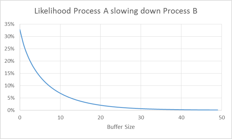
Please be aware that the detailed numbers in above graph are only valid for the above example, and if you have different means and standard deviations, your graph may look different. The general trend is true, however. A small buffer makes a big difference, whereas a larger buffer will not give you as much improvement.

Now, in theory you could do a cost benefit analysis to find your sweet spot between the cost and effort of a buffer size and its benefit for the overall system performance.

Fancy Math, But How Does This Help You on the Shop Floor?

Well, unfortunately it doesn’t help you on the shop floor! I have included the math above for two reasons. First, I wanted to show you that I can do math 😉 . The second and more important reason was to show you that the relation between buffer size and decoupling of processes is nonlinear. A small buffer is almost always sensible. However, making a large buffer even larger will not yield much additional benefit.

In practice, however, these theoretical calculations will not help you much. You rarely know the distributions of your processes well. Real world is also likely more complex, having more than two processes influencing each other. The above calculations are also rather complex, and not everybody can do these. In sum, the benefit of doing such detailed calculations are usually not worth the effort. However, if you really want to but don’t care about the math, then see my FIFO calculator.

FiFo Sizing on the Shop Floor

A Few Practical Suggestions

So how do you determine the size of a FiFo? In truth, there is not really any rule of thumb. As consultants we would have used an expert estimate – which are nothing but fancy words for the gut feeling of somebody familiar with the system. Hence:

To determine the FiFo size, ask somebody familiar with the system about his opinion. The FiFo should be able to cover failures, change-overs, or other downtimes of the processes, while at the same time be not too big and cumbersome. Adjust if the real behavior does not meet your expectations.

Disappointing, isn’t it? After all this math, I just tell you to pull it out of somebody’s a**. Yet that is current industry practice. However, there are a few more words of wisdom going around that I found helpful. The first one is:

Buffers are more important before and after the bottleneck(s) than they are around non-bottlenecks.

Buffering the bottleneck is sensible, since you don’t want your bottleneck to wait for other processes. Buffering non-bottlenecks is less useful, since they usually have to wait for the bottleneck anyway.

Add at least a buffer of one between processes when possible (if the cycle time of your processes is not linked, e.g., as with a conveyor belt).

One buffer will make the largest difference. Having one buffer between all processes will make the material flow much smoother. The exception is for systems with a identical tact time for the entire system (e.g., conveyor belts). The belt moves with the same speed everywhere, hence a buffer on the same belt is not needed. This also gives a rule for systems with linked cycle times:

If the cycle time of your processes is linked (e.g., as with a single conveyor belt), usually no buffers are needed.

Some Not-So-Useful Rules – Don’t Use!

There are some more rules out there, but many of them are pseudo-math. They calculate something and you get a result, but it bears little to no relation to the original problem you tried to solve.

For example, one rule defines the FiFo lane based on the desired lead time. If you want a long lead time, simply make your FiFo larger. But then, who would want a long lead time?!?!

Another rule defines the FiFo size for processes that require curing (i.e., a glue drying or a part cooling, etc.). The FiFo lane should be long enough so that the part can finish its curing process (including some safety time). Yes and no. Of course, there should be enough space so that all the parts fit, but curing is also an activity, not just a buffer. If you just put a FiFo there and hope it works, you will almost certainly end up with not-yet-cured parts downstream. For the sake of your quality, install a timer or something that makes sure all parts are fully cured before they move on.

Yet another rule looks at the shelf life. The FiFo should not be so long as for products to expire while in the FiFo. Theoretically absolute correct, practically totally useless advice. Or have you ever seen a FiFo longer than the shelf life?

Overall, FiFo sizing is still based much on experience. As always, I hope this post was interesting to you. Feel free to leave a comment below. Now go out and improve your industry!