
 This second post in a series on how to reduce your lead time looks deeper at the effect of fluctuations and utilization. Improving these will reduce your inventory and hence, as per Little’s Law, reduce your lead time.
Reduce Fluctuations
 Your inventory helps you to cover fluctuations. The next step would be to reduce fluctuations (in Japanese “mura“). This is also not easy. I recently did a multi-post series on how to reduce fluctuations in the source, make, and deliver side of your value chain. It is a Sisyphean task that never ends, since fluctuations always tend to increase unless they are actively reduced. The Kingman formula which I showed in the last post includes the fluctuations for the arrival and processing times, but this is a simplified model. In reality, you have multiple part types, multiple processes, and multiple queues. On top of that, the arrival of parts is often initiated by the departure, as in a pull system the departure of one part initiates reproduction. Hence, fluctuations in the demand pass through to fluctuations at the arrival.
Overall, it is hard to say how beneficial a reduction in fluctuations will be, but it will be beneficial. Hence, reducing fluctuations is an very important but underrated aspect of lean manufacturing.
 One fluctuation that affects the lead time especially is prioritization. If you have a priority “VIP” queue, the jobs in the VIP queue are prioritized and have a shorter lead time. This, however, comes at a cost of longer lead times of the non-VIP jobs. As long as you prioritize no more than 20%–30% of the work, the negative impact on the non-VIP jobs is negligible. However, the more jobs you prioritize, the worse the effect on the non-VIP jobs. Eventually, the non-VIP jobs may have a lead time approaching infinity.
With make-to-order, reduction in fluctuations help primarily with reducing lead time. With make-to-stock, the primary goal of reducing fluctuations is to reduce inventory, and a reduction in lead time is a nice side effect with additional benefits.
Reduce Utilization
 Another major factor in the Kingman equation is the utilization. As the utilization approaches 100%, the waiting time approaches infinity. The utilization is – indirectly – another way to manage fluctuations. There are three ways to decouple fluctuations, inventory, capacity, and time. Having a utilization of less than 100% gives you a capacity buffer to decouple fluctuations. If you want to have high utilization, you need lots of inventory in the system to reduce the chances of running out of material. Lots of inventory – you guessed it – means a long lead time. Hence, 100% utilization is a really bad target for a production system!
For one, your production system is not balanced perfectly, and some processes are needed more than others. It is absolutely normal and okay for non-bottlenecks to have less than 100% utilization. Even bottlenecks have less than 100%, since the bottlenecks usually shift. It also depends on how you measure utilization. Is it the percentage of the time a machine is scheduled for production? Or is it the ratio of the actually produced good parts to the maximum number of parts that could theoretically have been produced in the same time? This is better known as the OEE. Aiming for a 100% OEE is unrealistic (unless the number is fudged, and I have seen plenty of OEE claimed to be above 100%). Just as a reference, Toyota aims for around 90% OEE.
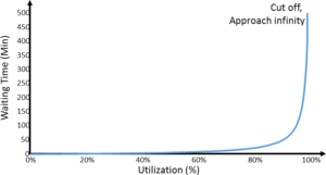
In any case, a utilization of less than 100% gives you a capacity buffer to handle fluctuations. You could also use inventory to decouple fluctuations. However, a capacity buffer does not increase your lead time, whereas inventory does. On the downside, a capacity buffer with workers and machines waiting for parts costs you too. The question is a trade-off between unused capacity and additional inventory. Furthermore, this trade-off is not linear as shown in this graph based on the Kingman equation. The closer you get to 100% utilization, the more inventory you need to cover even the smallest fluctuations. For an utilization of 100% you need – in theory – an infinite inventory. Please note that the graph measures only the waiting time for a simplified system with one queue and one process, but similar behavior can also be found in more complex systems.
Hence, reducing utilization a bit below 100% will save a lot of inventory and hence a lot of lead time. A sweet spot is often around 80%–90% utilization, although it depends on the details of your system. Reducing the utilization further has much less impact on the inventory and hence the lead time. For example, if you reduce your utilization from 60% to 40%, the impact on the inventory and lead time is negligible, but now your workers stand around even more, which costs money.

The Kingman equation gives a nice relation between utilization and lead time. But again, the Kingman equation is a simplified model of the real world. Regarding utilization, it assumes a round-the-clock non-stop working system. Such systems exist in reality. However, most systems do not work twenty-four hours a day seven days a week. Instead, you may have one shift or two shifts four, five, or six days per week. This gives you another way to use capacity for handling fluctuations, namely with overtime. Overtime where you call people in when you need them is cheaper than having them waiting around if there is no work. On the downside, overtime requires a bit of preparation, and hence can cover medium- or longer-term fluctuations like seasonality. Overtime can also handle fluctuations whose short-term effects were buffered by inventory. If you see your buffer inventory going down, you may schedule overtime.

But keep in mind that even with overtime, your utilization will not be 100%. Overtime cannot cover short-term fluctuations unless you have inventory. Trying to reach 100% utilization will again blow up your inventory and lead time. In sum, it is okay to aim for getting the most out of your system. But keep in mind that it will not have a 100% OEE, and that is okay. Also keep in mind that if you run your system around the clock like a paper mill or similar, you need an additional capacity buffer (a lower utilization) if you want a short lead time or a good product availability.
Hence, reducing fluctuations in general and utilization to a reasonable level will reduce your inventory and hence your lead time. Now, go out, reduce your fluctuations, manage your utilization, control your lead time, and organize your industry!
Series Overview
- Reducing Lead Time 1 – Inventory
- Reducing Lead Time 2 – Fluctuations and Utilization
- Reducing Lead Time 3 – Throughput and Lot Size
- Reducing Lead Time 4 – Development
P.S.: This series of posts is based on an inspiration by Rajan Suri, and also chapter 7 of his book Quick Response Manufacturing and chapter 3 from his book It’s About Time.
- Suri, Rajan. It’s About Time: The Competitive Advantage of Quick Response Manufacturing. 1 edition. New York: Productivity Press, 2010. ISBN 978-1-4398-0595-4.
- Suri, Rajan. Quick Response Manufacturing: A Companywide Approach to Reducing Lead Times. Portland, Oregon, USA: Taylor & Francis Inc, 1998. ISBN 978-1-56327-201-1.
Thank you Christopher for the two articles on reducing lead time. I have also been following up on your other articles.
One important factor regarding reducing utilization, is the rejection of the idea by the finance people. From my long experience working as the COO of a Group of manufacturing companies, the CFO and his team were always reluctant to any initiatives aiming at reducing utilization. However, I had notices that they would not mind a drop in utilization if it was an inevitable outcome resulting from a plummeting demand, but they would not accept any deliberate action, especially when it comes to expensive machines.
This might not be a problem in a small factory but it can be a source of conflict in large companies where the finance people have an influence on operational decisions.
Hello Mohammad,
for finance people it is a simple calculation, high utilization makes more parts and hence more profit. They can calculate this well. They can NOT calculate the bad effects of high utilization, and hence to them these bad effects don’t exist … but they do!
Thank you Chris for the 2nd part of the article . The 2nd part of the article related to utilisation of the capacity is very pertinent . There is almost a sense of obsession in terms of trying to utilise 100% of the capacity and in many cases it has been a challenge trying to explain to people – the negative consequences of this obsession, especially in a MTO environment – where Lead times elongate and delivery dates are not met, affecting credibility and eventually business prospects.
I would request you to dwell a little more on Inventory, Time and Capacity buffers. Thanks again for your insightful note
Hello Ramesh, have you seen my post on the “The Three Fundamental Ways to Decouple Fluctuations“? I go into more detail on inventory, time, and capacity.
Looking for the Actual values of OEE & UTILISATION IN a Press Shop with Progressive Dies. 3 shift Working for Bench marking.
Hello Reddy, find out what you have currently. Then try to improve it. Generally, utilizations of over 90% are to me risky territory, since eventually the negative effects start to become larger. In a job shop that would be more for the bottlenecks, but not for every process! But it depends heavily on your system!
I worked with an ex-stock manufacturer that amply demonstrated the impact of variability reduction, through Kingman, by adopting a genuine enterprise-wide pull replenishment process that replaced the (ubiquitous) forecast driven MRP mechanism built into their ERP/APS system. Instead of being driven by forecasts that were >40% wrong (thereby generating flow variability through constant schedule interventions) their end-to-end pull process enabled them to halve their factory lead-times, eliminate the 3rd shift (less unplanned machine change-overs = freed up capacity) and reduce inventory by 35% (despite now planning to hold it in the right locations) while achieving target service levels.
Hi Simon, great success story! Thanks for sharing!
Hi Christoph. Congratulations for your excellent web.
I think it is important to distinguish between utilization (Kingman), availability (OEE – TPM), and uptime (Lean).
Utilization is 100 minus the % of planned time when queue and equipment are empty (waiting for material).
Availability is 100 minus the % of the planned time in which the equipment is stopped due to breakdowns, changes and waiting (lack of material, lack of operator, lack of tools, etc.).
The uptime is 100 minus the % of the planned time that the equipment is stopped due to breakdowns.
It is possible to have a very high utilization (the queue is almost never empty) and yet an availability (and therefore OEE) and a uptime both awfull. It is the case in which losses due to breakdowns are very important.
The breakdowns increase the equipment utilization and mura of process time, and decrease OEE and uptime.
In the reverse case, a very high OEE always implies high utilization and high uptime.
Please, let me know if I am wrong.
Thanks.
Regards.
Hi Francisco, This is related to the OEE calculation, and also on how it is defined in your plant (there seem to be different definitions around, often designed to make the number look bigger and better). The OEE has three “losses”: Availability, speed, and quality. The basis of the OEE is the time the machine is scheduled to run (where some plants already argue to exclude maintenance). If you just take away the availability losses you would have the uptime (again depending on your definition).
Hi Christoph,
Thanks for your answer.
I have probably not expressed myself quite well.
Indeed, the OEE = Availability x Performance (speed) x Quality.
Seiichi Nakajima (Introduction To TPM) in his “Big Six Losses” does not mention where to include unplanned waits, such as:
– materials shortages (empty input queue)
– labor shortages
– lack of instructions
– lack of …
Each company that uses the OEE has its own criteria / calculations in this regard.
The consultant who taught me how to use OEE 20 years ago included in Availability (in addition to Breakdowns and Die Change) the unplanned waits mentioned above.
My comment was intended to highlight that in the Utilization calculation (Kingman / Rajan Suri / Spearman-Hopp) only the materials shortages time (empty input queue) is discounted.
Best Regards Christoph.
Hi Francisco, I see you use the multiplication approach to calculate OEE. I find the addition approach much easier (see my post Good and Bad Ways to Calculate the OEE). I would definitely include unplanned waiting times in the OEE losses. All the examples you listed are for me an OEE availability loss. I would even include planned stops like maintenance as long as it happens during regular work hour, but many companies like to exclude these to have a better looking OEE number.
The Kingman equation calculates the utilization as the mean time for service by the mean time for arrival. But the kingman equation is a theoretical model. I don’t think Kingman was looking at lack of material or quality defects when developing his formula. But I would agree with your interpretation that availability losses (stops) are used to determine the utilization. After all, a quality loss would still increase the waiting time, even if the part produced is thrown out afterwards.
Cheers!
Hi Christoph, I really appreciate your comments and your patience.
I understand and fully agree with all the clarifications regarding the OEE.
Regarding the utilization (u) of the Kingman equation (it is a theoretical model) I would like to comment one thing. I will borrow the notation used by Dr. Rajan Suri and the numerical example on page 77 (chapter 3) of his book “It’s About Time”.
Utilization (u) = TJ / TA, where
– TJ = mean working time (mean service time)
– TA = mean time between arrivals (mean arrival time)
As well:
Utilization (u) = Total time the machine is occupied / Total time the machine is scheduled to work
Example (CNC Lathe, page 77, It´s About Time, Dr. Rajan Suri):
– Scheduled time: 8 hours / day, 20 days / month = 160 hours / month
– Manufacture of parts (in cycle): 104 hours
– Setup: 26 hours
– Preventive maintenance: 3 hours.
– Breakdown (includes the time is waiting a maintenance person): 11 hours
– Utilization (u) = (104 + 26 + 3 + 11) / 160 = 144/160 = 0.9 (90%)
In this example, we could say:
– The machine has 160-144 = 16 hours a month (10%) of free capacity (could have taken extra work)
– Or, that for 16 hours a month (10%) the input queue and the CNC lathe have been empty
– Or, that the materials shortages represent 16 hours a moth (10%)
Of course, according to Kingman, we can reduce utilization, and therefore improve lead time, if we reduce setup time (26 hours) and/or reduce breakdowns (11 hours). In addition to the beneficial effect on variability of TJ (working time or service time).
Thank you very much Christoph
Hi Francisco, What you are saying sounds correct. Using the CNC example from Suri, there are 104 hours of the machine actually working, 40 hours of stops due to the system (Setup, maintenance, breakdown) and 16 hours of stops due to a lack of work. Other losses like quality and the hard-to-catch speed losses are probably part of the 104 hours machine time. For the kingman equation the utilization would need to include everything but waiting for work, hence the 90% utilization. The OEE would be less, as it has at least (26+3+11)/160 = 25% availability losses (using my preferred additive formula, not the multiplicative one). Even if quality and speed losses would be perfect, the OEE cannot be more than 104/160 = 65%.
Again, this would be the correct use in my opinion for the kingman equation with an utilization of 90%. Unfortunately, utilization is sometimes defined differently, hence in a new plant if you need the number you should check what is included.
Good Discussion!
Hi Christoph,
Completely agree.
Best regards.