
 In my last post I presented you Rajan Suri’s Power of Six – the relation between turnaround time and product cost. In this post I extend his work to apply it to not the entire value stream but to segments of the value stream. Enjoy!
Power of Six for Segments of Value Chain
 The Power of Six is used to calculate improvements across the entire value chain. As a recap, here is the Power of Six relation again from the previous post:
- C0 is the current product cost
- C1 is the desired new product cost
- T0 is the current turnaround time
- T1 is the new turnaround time needed
To consider the entire product cost, you would need to consider the entire value chain. The original source is a bit fuzzy on that, as they merely looked at the value chain underneath of their control, for products where this part of the value chain was the largest part of the value chain. Yet, considering the overall accuracy of the data this approach works.
But how do you approach if you only want to improve a small segment of the value chain? For example, if you have a series of kanban loops and want to improve only one loop. Take for example the simple system below.

A Couple of Reasons Why This Would Not Work
 Okay, I rarely do this, but let me get a bit academic and tell you all the things that should not work … before telling you later why, with respect to the accuracy of the Power of Six, it is good enough. So if you want, you can skip this section and jump to the next one for how it would work.
There are a couple of pitfalls here. First, for the kanban calculation, you do have the replenishment time. However, if you use the replenishment time, you ignore the time the material is waiting in the supermarket. This would have to be included.
Second, assume you want to improve the kanban loop D above. However, loop D is not part of the critical path. Improving loop D will not improve the overall turnaround time, which would be loop A, B, and C. The original Power of Six would consider here only improvements along loops A, B, and C. Yet, improving loop D will also be beneficial; it is just that the Power of Six rule can no longer calculate it.
You could also believe that the power of six would work for subsegments, where you relate the turnaround time for that segment T0,S and T1,S and its impact on the value add within this segment C0,S and C1,S, where
\[ { \frac{T_{1,S}}{T_{0,S}} = ( \frac{C_{1,S}}{C_{0,S}})^6}\]Mathematically speaking this relation is incorrect. First let me explain why this is so, before farther down telling you why it is good enough. Assume the total time T0 is the sum of the time of the segment T0,S you are improving and the time of the remainder outside of the segment T0,R. Similarly the total cost C0 is the cost of the value add of the subsegment C0,S under analysis plus the remaining costs C0,R . Similar applies to T1 and C1.
\[{ T_0=T_{0,S}+T_{0,R}}\] \[{ T_1=T_{1,S}+T_{1,R}}\] \[ { C_0=C_{0,S}+C_{0,R}}\] \[ { C_1=C_{1,S}+C_{1,R}}\]Hence the formula would be
\[{ \frac{T_{1,S}+T_{1,R}}{T_{0,S}+T_{0,R}} = ( \frac{C_{1,S}+C_{1,R}}{C_{0,S}+C_{0,R}})^6 = \frac{(C_{1,S}+C_{1,R})^6}{(C_{0,S}+C_{0,R})^6}}\]which would solve to something messy like
\[ { \frac{T_1}{T_0} = \frac{C_{1,S}^6 + 6C_{1,S}^5C_{1,R} + 15C_{1,S}^4C_{1,R}^2+ 20C_{1,S}^3C_{1,R}^3+ 15C_{1,S}^2C_{1,R}^4+ 6C_{1,S}C_{1,R}^5+C_{1,R}^6}{C_{0,S}^6 + 6C_{0,S}^5C_{0,R} + 15C_{0,S}^4C_{0,R}^2+ 20C_{0,S}^3C_{0,R}^3+ 15C_{0,S}^2C_{0,R}^4+ 6C_{0,S}C_{0,R}^5+C_{0,R}^6}}\]and definitely not into something nice like the formula we had a little bit earlier
\[ { \frac{T_{1,S}}{T_{0,S}} = ( \frac{C_{1,S}}{C_{0,S}})^6}\]Hence, purely mathematically speaking, this approach would not work. But see farther down below.
The Correct Approach Using the Power of Six
If you improve only a segment of your value stream, and if this segment is on the critical path, you would have to estimate the share of your improvements with respect to the entire turnaround time to get an estimate of the improvement of the entire cost.
Let’s take the example below. You improved segment B in your value stream, reducing the turnaround time for this segment from six days to four days, improving it by two days. Since the entire turnaround time across the value stream is twenty days, your overall improvement is still only two days, and the new turnaround time comes down to eighteen days.
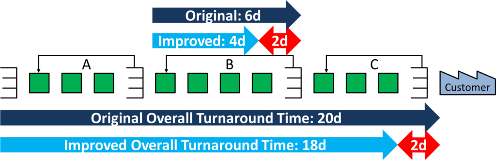
Hence your overall reduction of the turnaround time was by 10% to 90% of the original value, and your cost should go down by around 1.74% to 98.26% of the original value as shown below.
\[ { \frac{C_1}{C_0}=(\frac{T_1}{T_0})^ \frac{1}{6}=(\frac{18}{20})^ \frac{1}{6}= (90\%)^ \frac{1}{6}= 98\%}\]This approach would work, although it requires you to understand the turnaround time for the entire value stream, which may sometimes be tricky. It also does not work for subsegments that are not along the critical path (as for example segment D in the example farther up).
A “Good Enough” and Practical Estimation
![]() A little bit earlier I introduced you this equation, and told you that it is not mathematically proper. Here it is again and also its reverse from:
A little bit earlier I introduced you this equation, and told you that it is not mathematically proper. Here it is again and also its reverse from:
However, I am not an mathematician but an engineer, and 1+1≈2 is often good enough for me. And, luckily, this equation is good enough for pretty much all cases. Let’s compare the accuracy of this equation for a segment with the “correct approach” based on the improvement of the total turnaround time above.
Let’s take the example from above again and assume your total turnaround time is twenty days. You optimize one six-day segment of your entire value stream to reduce your turnaround time by two days to four days (i.e., the total improvement would reduce turnaround from twenty to eighteen days). Using the Power of Six properly, this would estimate a cost improvement of 1.74% to a new cost of 98.26% (and I am aware that this number of digits is excessive for the accuracy of the method).
If we look only at the section itself, we have a reduction by two days from six to four days. This would reduce the cost in this segment by 6.53% to 93.47%.
\[ { \frac{C_{1,S}}{C_{0,S}} = ( \frac{T_{1,S}}{T_{0,S}})^ \frac{1}{6}=( \frac{4}{6})^ \frac{1}{6} = 66.66\%^ \frac{1}{6}=93.47\%}\]If we assume a linear relationship of the cost and hence assume that this segment that has six of the twenty days turnaround time has also 6/20th of the cost, then we can estimate the overall cost improvement as follows:
\[ { 1-\frac{C_{1,S}}{C_{0,S}} = ( 1-(\frac{T_{1,S}}{T_{0,S}})^ \frac{1}{6}) \cdot \frac{T_{1,S}}{T_{1}} =(1-93.47\%) \cdot \frac{6}{20} = 6.53 \% \cdot 30 \%= 1.96 \% }\]So overall, the “correct” approach would give us an improvement of 1.74%, and the simplified approach would give us 1.96%. For me this is good enough, especially considering the accuracy of the method.
Just to make sure that this is not a fluke, I tested different improvements with different shares of the overall value stream. Unless you manage to eliminate nearly 100% of the time in your segment, the overall estimate is to me close enough. I tested an overall improvement of 10%, 30%, 60%, and 90% for different shares of the segment of the overall turnaround time. This is shown below, where I compare the segment based calculation with the correct approach (the red lines).
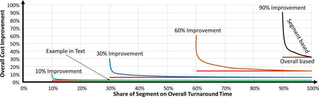
Naturally, if the overall improvement is 60%, the segment cannot be less than 60% of the overall. Even then the segment would have to reduce its time to zero to achieve an overall improvement of 60%. Hence the graphs below always end on the left side.
It can clearly be seen that unless you eliminate a segment completely, the segment-based calculation and the overall approach have rather similar results, again considering the accuracy of the method. Hence this “good enough and practical” application of the power of six is probably good enough for your cases. An additional benefit is that this segment based approach allows the calculation of the improvements of segments not on the critical path. In this case you merely calculate the improvement for the value add based on this part of the segment.
Conclusion for Segments
Hence you can use the Power of Six rule also for segments. The equation would stay the same, you merely apply it to part of the value stream.
- C0,S is the current value add in your value stream segment
- C1,S is the desired new value add in your value stream segment
- T0,S is the current turnaround time for your value stream segment
- T1,S is the new turnaround time needed for your value stream segment
The relation according to the power of six is as follows:
\[{ \frac{T_{1,S}}{T_{0,S}} = ( \frac{C_{1,S}}{C_{0,S}})^6}\]or in its inverse form
\[ { \frac{C_{1,S}}{C_{0,S}} = ( \frac{T_{1,S}}{T_{0,S}})^\frac{1}{6}}\]How to Get There?
You can start with a financial target and estimate the needed reduction in turnaround time, or you can start with the reduction in turnaround time and estimate the financial benefits. In any case, you would need to reduce turnaround time eventually. This, of course, is not that easy (otherwise you would have done it already). The full extent of your options would exceed the scope of this post, and I have written about this in many other blog posts. See A Eulogy for Little’s Law, How Product Variants Influence Your Inventory, How to Reduce Your Inventory, and many more. But somehow you need to get your turnaround time down.
I hope this post was not too mathematical for you. Now, go out, reduce your turnaround time, estimate the benefits using the Power of Six, and organize your industry!
P.S.: Many thanks to Rajan Suri for his input and help, and of course for finding this relation in the first place!
Sources
- Suri, Rajan. It’s About Time: The Competitive Advantage of Quick Response Manufacturing. 1 edition. New York: Productivity Press, 2010. Pages 165–167.
- Suri, Rajan. MCT Quick Reference Guide. Suri Consulting and Seminars, LLC, 2014. Page 11.
- Tubino, Francisco, and Rajan Suri. “What Kind of ‘Numbers’ Can a Company Expect After Implementing Quick Response Manufacturing? – Empirical Data from Several Projects on Lead Time Reduction.” In Quick Response Manufacturing 2000 Conference Proceedings, 2000.