
 The lead time of a system is heavily influenced by both the utilization and the variation. There are approximations available to estimate this relation, and one of them is the Kingman formula. In this post I would like to introduce you to this equation and describe the fundamental understanding of it. Luckily, you don’t really need the formula for your daily dose of lean. The equation itself has little practical use. However, this relationship is important for understanding the behavior of your production system. While you won’t use the Kingman formula to evaluate your production system, understanding the equation will help you in tweaking your system in the right direction.
Lead Time
 The lead time is the time it takes for a single part to go through the entire process or system. This is an important measure of the speed at which the system can react to changes. If you introduce new products or product changes, the lead time is (on average) the time until these changes come out at the other end. If your customer orders a custom made-to-order product, this is the (average) time your customer has to wait.
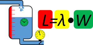
Hence, a lean production system aims to reduce the lead time. It is easy to determine the lead time for an existing system. You simply use Little’s Law. There are three variables, often labeled as follows:
- L – Inventory, measured, for example, in units or quantity
- λ – Throughput, measured in units or quantity per time
- W – Lead time, measured in time
Little’s Law is then the simple relation shown below:
\[{ L= \lambda \cdot W} \]While Little’s Law tells you the lead time, it does not tell you much about how to influence it. Obviously, the main lever is to reduce your inventory (if you are active in lean manufacturing, you may have come across this idea 😉 ). Yet, in most cases this inventory is there for a reason, mainly to buffer fluctuations (but also others, see my post Why Do We Have Inventory?).
The Kingman Equation
The Kingman equation (also known as Kingman formula or Kingman approximation) gives you an approximation of the waiting time of the parts for a single process based on its utilization and variance. It was developed by British mathematician Sir John Kingman in 1961. As shown in the image, the parts arrive randomly, with a mean time μa between arrivals and a standard deviation σa. The parts then wait in the queue until they are processed (i.e., serviced). The service time has an average duration of μs and a standard deviation of σs. The equation determines an estimation of the waiting time (excluding the part in the process).

The equation includes the following variables, commonly written as:
- E(W): The expected waiting time W.
- μa and σa:Mean and standard deviation of the time between arrival of parts. This includes the losses. I.e. it would be NOT the cycle time, but rather the arrival takt time.
- μs and σs:Mean and standard deviation of the time to process one part. Please note that this usage is not standardized, and some equations use the symbol μ for the service rate, which would be the inverse of the mean time to process one part. Similar to the arrivals, this would also include the losses and hence be themean and standard deviation of the process takt time.
- p: Utilization (i.e., the percentage of the time a machine is working). It is calculated by dividing the mean time for service μs by the mean time between arrival μa. If the arrival is faster than the service, you would have an utilization above 100%, which is not possible. Hence μa has to be smaller than μs. Therefore, p can range from 0 to 1. (Note: If the parts arrive faster than they can be processed, then the waiting time will go toward infinity. Even if the arrival is exactly equal to the service, the waiting time will still go toward infinity.)
- ca: The coefficient of variation for the arrival (i.e., the standard deviation σa divided by the mean μa for the time between arrivals).
- cs: The coefficient of variation for the service (i.e., the standard deviation σs divided by the mean μs for the average duration of a service).
Please note that the Kingman equation requires independently distributed arrival and service times (which is usually valid for most manufacturing systems), and is valid only for higher utilizations (which is also often true in manufacturing). Please note that this is also only an approximation, not a precise formula. And finally, it is only for a single arrival with a single process, which is quite rare in practice.
An Example
Let’s look at an example. We have an arrival process with an average of 10 minutes between parts and a standard deviation of 8 minutes. Our service needs, on average, 8 minutes per part, with a standard deviation of 7 minutes. We have an utilization of 8/10 or 80%. Or coefficient of variations are: ca = 8/10 = 0.8 and cs = 7/8 = 0.875. Hence the equation is as follows, giving an expected waiting time of 22.49 minutes:
\[ { E(W) = \left ( \frac{0.8}{1-0.8} \right )\cdot \left ( \frac{ 0.8^{2} + 0.875^{2} }{2} \right ) \cdot 8 = 22.49 Minutes } \]Again, this is only an approximation. The results depend heavily on the type of distribution. Using simulation for verification, actual waiting times were 20.8 minutes for Lognormal distributions, 21.19 minutes for Weibull distributions, and 18.16 minutes for the Pearson Type V distribution. Especially the Pearson Type V had a larger error, presumably because this distribution is heavy tailed compared to the others.
Interpreting the Formula
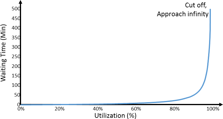
This equation (or more precisely, this approximation) shows us the two factors that influence your lead time and your queue length. One important factor is the utilization. The higher your utilization, the longer your queue. Eventually your queue will approach infinity as your utilization approaches 100%. This would be the first bracket of the equation above. The graph below shows the waiting time for different utilization for the example above. The closer you get to 100% utilization, the closer you will get to an infinite queue length.
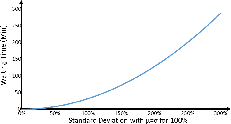
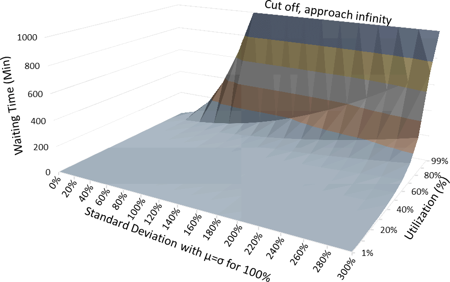
The second factor is the variation. The higher your variation, the longer your queue. This would be represented by the right bracket in the equation above. The image below shows this relation again for our example above. The standard deviation was varied from 0% of the mean to 300% of the mean. You can see clearly how the waiting time increases.
Finally, these two parts are not added but multiplied with each other. Hence, while a high value in each is not good, a combination thereof is even worse. This is visualized in the chart below.
What Does This Mean?
This means, most of all, two things if you want to have a reasonable lead time or queue length:
- Stay away from 100% utilization. The lower your utilization, the shorter your lead time. Of course, a higher utilization also means a better use of the invested capital. Here you have to make a trade-off between a good usage of your machines with high utilization and a low lead time with low utilization.
- Try to reduce variation. Lower variation allows you to get away with lower inventories. Of course, this is easier said than done. The idea of leveling in lean manufacturing aims to reduce this variation to obtain faster lead times and other benefits.
- If you have high variability, try to use lower utilization. If your workshop has a high demand on flexibility, you can ease the pressure by reducing the utilization.
- If you have high utilization, try to reduce variability. If your workshop has a very high utilization, it may help to reduce the variability, although this is often easier said than done.
Alternative Calculations
The Kingman formula is the best known version to estimate waiting time, but by far not the only one. In the 1960s, lots of researchers developed formulas, some of which were more precise but a bit more cumbersome to handle. (For sources, see below.) W. G. Marchal published the following formula in 1976:
\[{ E(W) = \left ( \frac{p ^2 \cdot \left ( 1 + C_{s}^{2} \right ) }{1+p^2 C_{s}^{2}} \right )\cdot \left ( \frac{ C_{a}^{2} + p^2 C_{s}^{2} }{2\cdot \left ( 1-p \right )} \right ) \cdot \mu_{s} } \]Almost simultaneously, Kramer and Langenbach-Belz published the following formula also in 1976:
\[ { E(W) = \left ( \frac{p ^2 \cdot \left ( C_{a}^{2} + C_{s}^{2} \right ) e^g }{2\left ( 1-p \right )} \right ) \cdot \mu_{s} } \]where
\[{ g= \frac{ -2 \left ( 1-p \right )\left ( 1-C_{a}^{2} \right )^2}{3p \left ( C_{a}^{2} +C_{s}^{2} \right )} } \]Both formulas are (reportedly) a bit more precise, but also not as nice to show the effects of variation for our purpose.
Of course, if both your arrival and your service distributions are exponentially distributed (known as a M/M/1 queue in the queuing theory), then the following equation is a precise calculation. Unfortunately, you cannot make this assumption in the real world.
\[ { E(W)= \frac{ p^2}{1-p} \cdot \mu_{s}} \]Anyway, this is all the math for today. Again, the formula is of little practical use, as it is only for a single arrival and a single process with an infinite queue, but the relationship it shows is important. The formula can also be used for single arrival and single process for batches of parts or job orders. In sum, stay away from very high utilizations, and from high variability if you can. Now, go out, find your trade-offs to control your lead time, and organize your industry!
Sources:
- Kingman, J. F. C.: “The single server queue in heavy traffic.” Mathematical Proceedings of the Cambridge Philosophical Society. 57 (4): 902. October 1961
- Marchat, W. G.: An approximate formula for waiting time in single server queues, AIIE Trans. 8(1976)473.
- Kramer, W. and Lagenbach-Belz: Approximate formulae for the delay in the queueing
system GI/G/1, Congressbook, 8th Int. Teletraffic Congress, Melbourne, 1976, pp. 235.1-235.8.
Have you heard of Big’s Law? It is the reverse of Little’s Law and measures the number of inventory turns.It is defined as the ratio Throughput/Inventory and is very well known.
This is, obviously, a bad joke. I leave up to you to publish this comment.
The rest of the post, as usual, excellent.
Kind regards.
Good article. Just sent toi my MBB to review this and look from different point of view for some of the issues on warehouse.
Hi Chris,
References to Kingman are always welcome in production! Wrote about the same topic July 2016. I have even tried to put in some more lessons and a link to a simulation on the web where you play with some parameters to experience the effects. You can find my post about it here: http://dumontis.com/2016/07/muri-mura-kingman/
MfG, Rob
Great article Chris. See also https://www.linkedin.com/pulse/supply-chain-flow-what-why-how-simon-eagle/?published=t on similar theme.
Hello Rob & Simoneagle, good posts on the topic by you, too. Without knowing I even used a similar cover picture as Rob. Interesting coincidence!
Hello Chris,
Excellent web and great post.
Perhaps it might be interesting to point out: 1) that the Kingman formula is applicable to both parts and batches/jobs and 2) that in the calculation of “μs” and “cs” must include the time lost by reference change, breakdowns, reprocessing, lack of operator in the service (sources of the service time variation).
Hello Francisco, Good Points. I added these good points to the post above. thanks for the input 🙂
All your formulas for alternative calculations use Mu_a. However, in your equation for the Kingsman’s approximation, you used Mu_b. I think the correct result for the Kingsman should use, just like all the other approximations, Mu_a.
In Wikipedia shows Mu_b, but in other papers, it shows as Mu_a.
Since Little’s law is
W=L x M_a
I would think maybe the right answer is to use M_a
Alberto: You are correct! I just checked my original Marchal paper, and he only calculates the waiting time, not the queue length, hence without the mu’s. For the queue length the mu-s is obviously correct. Thank you very much for picking up that mistake!
Hi Chris,
You mention Little’s law in you article and I am curious to know what the difference is between Little’s Law and the Kingsman formula, mainly the purpose of both. Am I right to say that Little’s law is showing the correlation between WIP and Flow? And Kingsman formula looks at waiting times taking utalisation & variance in consideration? Would Little’s Law more suitable for multiple services and variances?
Hello,
I have one doubt: let’s assume that it is not possible to reduce variation. If there are several sequenced workstations and we want to reduce utilization, process time1 > process time2> process time3>…
So the line takt time is defined by workstation1?
If there are 20 workstations, there should be progressive process time reduction one workstation after the previous?
Hi Hector, the line takt depends on a lot of things. One is the bottleneck process. But this is also influenced by fluctuations, which causes bottlenecks to shift between processes. This in turn is also influenced by inventory buffers between processes. The line takt is best measured directly, as it is hard to make a theoretical calculation.
Hi Christoph, working in IT the comparison with Lean manufacturing is interesting. I came across this article (https://fred.stlouisfed.org/series/MCUMFN) that, from what I understand, says that the capacity utilization in manufacturing is about 75%. I was wondering if that should be interpreted as that 25% of the time workers in factories are waiting? Or is it rather that companies are only utilizing 75% of their factories capacity, and to get to 100% they would need to bring in more people?
I realize you may not be fully aware of the data that the graph is based on, but what is your experience from having visited lots of factories?
Hi Dennis, capacity utilization usually refers to machines, not workers. It is also a question on how it is defined. It could be that the machines make 75% of what they could do in theory (I.e. OEE), but more likely the machines are running 75% of the time, including waiting for material and small breaks.