
 One of the most significant fundamental relations in lean manufacturing is the relation between the inventory, the throughput, and the lead time. The inventory and the throughput are usually easy to measure. The lead time, however, is more difficult. You would need to take the time when a part enters the system and then take the time again when a part leaves the system. Luckily, the lead time can easily and accurately be calculated using Little’s Law, one of the most fundamental laws in lean manufacturing (and also many other places).
Little’s Law was first published around 1954. It is named after John Little (an MIT professor and not one of Robin Hood’s merry men 🙂 ). He did not invent the law, but he was the first to mathematically prove the universal validity of it in 1961.
The Variables
First, let’s first explain the variables. Throughout this post, I will use a supermarket checkout as an example, assuming that all of you have at one time or another waited in line at the checkout. Hence, our example system is the checkout system, defined as the system including all customers waiting in line or being processed (but not still shopping for goods).
Inventory

Inventory is simply the number of parts in the observed system. You could also call it WIP (Work in Progress). For our supermarket checkout, the inventory would be the number of people waiting in line, including the customer currently being served (but not the cashier – that would be the process).
The inventory is usually quite easy to measure. You simply count the number of parts in the system, either by hand or by looking up your ERP data. You could use the current inventory if you are interested in a current state of the system. You could also use the average inventory over a longer period if you want to analyze the average behavior of the system.
Throughput
The throughput is the average number of parts completed in a given time. Taking again the example of a supermarket, it could be measured in customers per hour.
The throughput is also rather easy to measure. You check how many parts you have produced during a period of time. Dividing the number of parts by the total time gives you the throughput.
As for the throughput, again there are different ways you could measure it. You could look at a longer period, including weekends and off-shift times (i.e., how many parts did you produce during the month?). Alternatively you could only observe during actual working hours (i.e., how many parts did you produce during an 8-hour shift?). Both are possible. Depending on which one you use, you will get the throughput time in working hours or total hours including off-time.
Lead Time
 The lead time is the time a part takes to pass completely through the system (i.e., it is the time between entering and leaving the process). In the example of supermarket checkouts, it is the time from when you start to wait in line until you pick up your goods and leave.
The lead time is difficult to measure directly. In a supermarket, you could have everyone measure their own waiting time. For physical parts, however, someone would have to measure it. In reality, this is quite impractical.
The lead time, however, is an important value in manufacturing. A longer lead time means that you will need more time to implement changes.
Little’s Law
The Law
Little’s Law is actually quite simple. There are three variables, often labeled as follows:
- L – Inventory, measured, for example, in units or quantity
- λ – Throughput, measured in units or quantity per time
- W – Lead Time, measured in time
Little’s Law is then the very simple relation as shown below.
\[ { L= \lambda \cdot W} \]However, for sake of clarity I prefer to write it out in full. Hence:
\[{ Inventory= Throughput \cdot Lead Time} \]Hence, to determine the lead time you calculate:
\[ { Lead Time = \frac{Inventory}{Throughput}}\]And finally, to determine the throughput you calculate:
\[ { Throughput= \frac{Inventory}{Lead Time}} \]The Underlying Assumptions
Often in academia, you can find very boastful research results – except if you read the assumptions closely, you find out that it applies only to a very special and highly unrealistic situation. Quite frequently, these limitations make the research results unusable in practice.
Little’s Law, however, has only two major assumptions. First, you need to have a stable system without major changes. In other words, the three variables involved (inventory, throughput, and lead time) do not change significantly while being observed. Assume again you have a supermarket with one cashier. Using Little’s Law, you calculate the estimated waiting time based on the speed of the cashier and the number of people in the queue. However, if a second checkout line is opened, the speed of the system doubles. Hence, your calculation is no longer valid, since the system speed has doubled. Similarly, if the queue gets longer because more people arrive than leave, then Little’s Law no longer gives the average waiting time. Therefore the arrival and the departure rates have to be similar.
Second, the units used for the inventory, throughput, and lead time have to be consistent. Measuring the throughput in batches per hour, the inventory in individual items, and the lead time in days will mess your calculations up, unless you convert the values into consistent units.
In practice, however, both assumptions are very reasonable assumptions. First of all, most manufacturing systems do not change drastically within a short time, even if you merely update the values for the formula and get the new numbers. Regarding the units, basic knowledge of math and common sense can easily avoid this problem. Therefore, Little’s Law has an almost universal validity and is highly applicable in practice!
What Is Not Relevant
The beauty of Little’s Law are all the factors that do not matter. This universality makes Little’s Law extremely practical in everyday shop floor operations.
- Random distribution of the arrival and the departure speeds (the throughput): Regardless if you have normally distributed variables, exponentially distributed variables, or any other random distribution, Little’s Law holds true.
- Sequence of the material processing: No matter if you have FiFo (First in First out), LiFo (Last in First out), or any other or even a random sequence in your material flow, Little’s Law is valid to calculate the mean values! Of course, depending on your sequence, the fluctuation in throughput time may be much more in LiFo than in FiFo, but the mean is correct.
- Size of the observed loop: Again, it does not matter if you look at one machine, the complete manufacturing line, the entire plant, or even your entire logistics network. Little’s Law is valid!
- Everything else you can think of: As long as the two conditions above hold true, Little’s Law is valid!
Some Example Calculations

Let’s do some sample calculations. Assume a supermarket checkout line. How long does a customer have to wait at the supermarket checkout for the following example:
- L: 5 customers waiting in line
- λ: 2 customers leave the checkout per minute
Hence a customer waits an average 2.5 minutes in line. Let’s expand this for the entire supermarket. How long does the average customer spend in the supermarket? Let’s assume:
- L: 30 customers in the supermarket
- λ: 2 customers leave the checkout per minute
Hence the average customer spends 15 minutes in the supermarket, of which he spends 12.5 minutes shopping and 2.5 minutes at the checkout. If we observe the people more closely, we would also see that 25 of them are shopping and 5 are waiting at the checkout.

Let’s do a manufacturing example. What is the average duration a part spends in the finished goods warehouse (i.e., what is our reach on finished goods)?
- L: 10,000 pieces are in the warehouse
- λ: 15,000 pieces are sold per month
Hence the average piece spends two-thirds of a month in the warehouse. Let’s look at the lead time of the entire material flow:
- L: 15,000 units are in the system (of which 10,000 are in the warehouse, and 5,000 in various stages of completion)
- λ: 15,000 pieces are sold per month
Hence a part takes roughly 1 month to pass through the entire system. Now let’s assume we have a kanban system. How long takes a kanban to complete the loop? Assume one kanban represents 100 pieces, and there are in average 50 kanbans waiting for production.
- L: 20,000 finished and semi-completed units and planned units in the form of kanban are in the system (of which 10,000 units or 100 kanban with 100 parts each are in the warehouse, 5,000 units or 50 kanban are in various stages of completion, and 5,000 are represented by 50 kanbans waiting for production)
- λ: 15,000 pieces are sold per month, or the equivalent of 150 kanban with 100 pieces each
Hence it takes 1.33 months before a kanban completes an entire loop.

You can also use Little’s Law for continuous processing as, for example, chemicals. Let’s calculate how long water stays in America’s largest lake, Lake Superior, before it leaves the lake.
- L: 12,087.73 cubic kilometer (km3)
- λ: Water outflow is adjusted and varies throughout the season, but let’s assume it is 2,400 cubic meters per second (m3/s), which is 75.68 km3 per year
Hence water stays in Lake Superior for almost 160 years before it flows out. More than half of the water in the lake was already there when Abraham Lincoln was President 🙂 .
Why It Is Relevant
Little’s Law is almost always valid and very easy to calculate. It also shows the relation of the two factors influencing the lead time: inventory and throughput. The graph below shows this relation in relative terms.
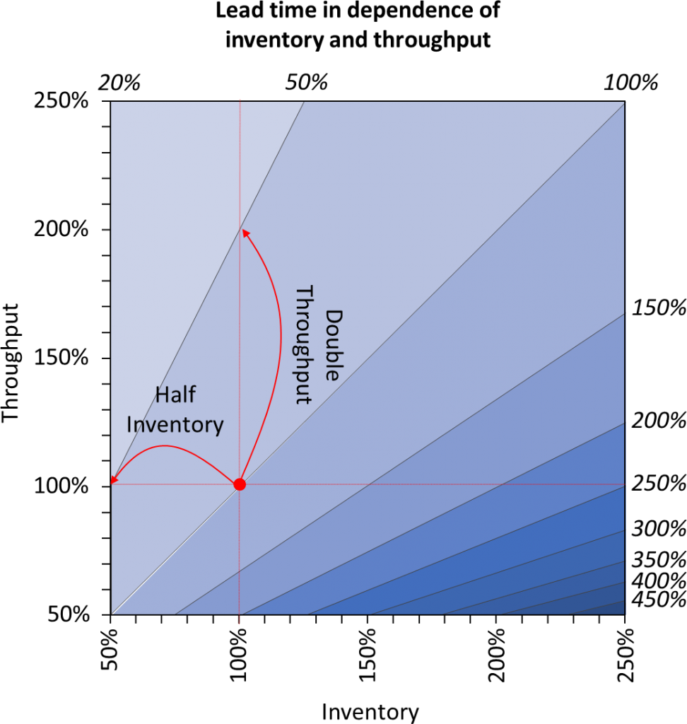 Hence, if you want to reduce your lead time by half, you would have to either double your throughput or halve your inventory. Both would achieve the same results. However, doubling the number of parts produced in a given time is probably rather difficult and expensive in practice. Halving the inventory is usually much easier. Besides, if you halve your inventory, you may even get money back by temporarily selling more than you purchase or produce.
Therefore, Little’s Law is another mathematical justification for the push in lean production to reduce inventory, and the advantage of pull production and its fixed limit on WIP. But please, keep enough inventory for your system to work smoothly, or it will be more expensive than before.
I hope this article was interesting for you and helps you with your daily work of improving your system. Now, go out, calculate your lead time, and organize your industry!
PS: This is my 100th post on AllAboutLean.com. Thanks for reading, following, and commenting 🙂
Thanks, very useful your posts.
You are a leader!
Hello ingfl, thanks for the praise 🙂
Thanks a lot , very clear !
Sandro (Bologna, Italy)
Thank you, Sandro 🙂
excellent explanation. thanks.
Thanks for the post. Simple analogy helped to get it better.
Thank you Spyros and Dhanesh 🙂
So one question. If I reduce the lead time, can I assume I increase the throughput and reduce the wip?
In other words, if i do a Kaizen to improve the throughput Is the lead time reduced?
Lead time, throughput and WIP are directly correlated. If you change one, you also change one or both of the other two. The usual way, however, is to reduce WIP in order to improve the lead time while keeling the throughput constant.
Of course you can also do the approach you described by improving throughput. However, this is often more difficult to do. Additionally, improving throughput also has other effects, e.g. possibly putting supply and demand out of balance. The parts will flow faster through your system and then pile up in front of the customer. Hence you may have created a local improvement, but worsened the overall situation. Happens way too often in manufacturing…
Of course if your supply is unable to meet demand you should increase throughput, although the improved lead time is in this case only a beneficial side effect of your main target to deliver to the customer 🙂
Thanks a lot for this very nice explanation,
Great Article..It was very informative..I need more details from your side..include some tips..I am working in Cloud Erp In India.
I’m confusing: How a kanban takes 1.33 months to complete an entire loop?
there are only 50 kanbans ( 50×100 parts) to supply 15000 parts for customer.
Hi Michael, i added units to the equation above for clarity. hope this helps, I should have done this in the first place. Cheers, Chris
Hello Christoph, I am not sure that I understand the value of using lead time reduction as a goal, as in the statement “Little’s Law is another mathematical justification for the push in lean production to reduce inventory”.
It makes sense to me that an increase in throughput benefits the company (more product sold/processed/etc. in a given time), and that, in the case that inventory stays constant, a reduced lead time indicates a higher throughput. But I am not sure that I see the benefits in all situations – for example, with a constant throughput, a reduction in inventory also gives a reduced lead time, but are the benefits of reduction in inventory mostly storage costs? If so, shouldn’t the formula be amended to drop out production time, and use storage time, not total lead time?
Do you count reducing wages, material, and other costs associated with producing the stored inventory as benefits, here? But if that inventory would need to be made eventually anyway (I guess here I am making an assumption to my specific situation, where production changes that result in discarding stock effectively never happen), are those benefits real, or just time-delayed?
Thank you very much,
Adam
Hi Adam, if you assume a near constant output (which is common, with growth rates per year of +/- 5%), then the only way to reduce your inventory is to reduce your lead time, and vice versa. Of course if you can sell more, go for it and try to keep your inventory the same – but in this case you must reduce lead time to maintain the same inventory. IN lean philosophy, inventory is one of the wastes. And inventory can cost you easily 30-70% of its value per year. Hence, if you have an inventory of 1 million$ it costs you 300.000-700.000$ per year just to have it. (see The Hidden and not-so-hidden costs of Inventory). Reducing lead time is next to reducing fluctuations one of the main levers to reduce inventory, which in turn is one of the main levers to reduce cost. Hope this helps, happy holidays, Chris 🙂
Thanks for your informative article.
However, I disagree with your last point “Why It Is Relevant”.
We can use Little’s Law when looking backward not for predicting the future. As you correctly mentioned in your article, when you change the system, we violate the assumption of stability.
This is an interesting article about it:
http://www.vissinc.com/2012/09/07/littles-law-isnt-it-a-linear-relationship/
Hi Analica, thats why “you need to have a stable system without major changes”. If the system changes in the future, then of course your outcome changes.
Hi Cristopher,
In our company while creating VSM, we do calculate LT between process this way :
LT = Inventory / Average Customer demand (Final Customer)
Example: Average customer demand/ day = 500 pieces (Customer demand and not machine Throughput)
Inventory: between process A and B = 5000
LT = 5000/500= 10 days
Or LT in raw material warehouse is calculates so:
LT= number of pieces in stock / customer demand
As we have an EPEI of 10 days that’s mean we do produce a big batch once in two week.
And so one between B and C till the shipping area or Stock.
And the total production leading is the addition of all LT between process + different cycle time in each process.
Does it make sense such calculation because it’s completely different of your way of calculation.
Thanks, in advance
Hi Alaeddin, this is absolutely correct. See the formula below “Hence, to determine the lead time you calculate:” above. You divide your inventory (5000 pieces) by your throughput (500 pieces per day) and get 10 days lead time. Cheers 🙂
Hi Mr. Roser,
Many thanks for your informative post. I was so happy when I read your PS, I still have 99 posts to read and enjoy 🙂
I am not sure that I understand the meaning of lead time, like in the first example (5 customers waiting in line, throughput = 2 customers/min), I think 2.5 min is the time needed to serve all the waiting customers. only the last customer will be waiting for 2.5 min. so, why you consider it as the average waiting time?
Another question please, how can we reduce the inventory (System level) in the supermarket question in order to reduce the lead time?
Thanks again.
Hi Summer, assuming a stable system, then the first person in line already waited for 2 minutes. Every new customer arriving has to wait 2,5 minutes. If you continue indefinitely, the average waiting time is 2,5 minutes. Only if you have 5 customers in line when the store (checkout) opens and no new customers come in then you will have an average of 1,25 min waiting till the line is empty.