
 Job shops are, in their nature, much more chaotic than flow shops. Previously, I have written a lot on this topic. In this post I would like to take a deeper and quantitative look at this effect. Using simulations, we take two systems and try to make them as identical as possible – except that one is a flow shop and the other is a job shop. This blog post is based on a thesis by my student Daniel Ballach.
The Two Systems
The goal was to make two systems as identical as possible. The flow shop was the easy part. You just have a sequence of processes with FIFO buffers in between. Below is an example shown with 5 processes, although we varied the number of processes between 1 and 50. The processes had all the same cycle time of 10 time units, randomly distributed using a gamma distribution. In front of every process was a FIFO with a maximum capacity of 10 parts. Both supply and demand was infinite.

For the job shop, we kept the system as identical as possible, except the routing was changed. Every arriving part was randomly assigned to one of the different processes. A counter tracked how often a part has been processed already. After 5 iterations, the part leaves the system. This gives the same workload as with the flow shop. Parts that have not yet been processed 5 times go back to the random process assignment. Parts that come back have priority over parts that have not yet been processed at all. To avoid blocking situations, these parts that have been processed at least once may have to wait in a separate queue before the prioritization and random assignment. Similar to the flow shop, we also simulated systems between 1 iteration with 1 process and 50 iterations with 50 processes.
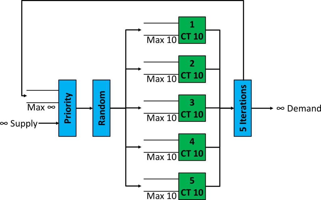
The additional queue for the parts looping back will slightly increase the inventory, and hence the lead time. However, this was necessary to avoid blocking.
Utilization and Line Takt
Let’s first have a look at the utilization. The blue line in the graph below is the average utilization in a flow shop. Again, all processes have the same cycle time distribution, meaning they all have the same speed. With a large buffer in between, these processes can work pretty much full-time, with utilizations ranging from 99.6% to 99.9%. Longer flow shops have very slightly lower utilization, although it does not make much difference. Of course, in reality your processes would have slightly different cycle times, you would have breakdowns, and your buffers may not be quite as large, resulting in lower utilizations.

The utilization in the job shop, however, showed a significant decline as the number of processes increased. The largest system with 50 processes had an utilization of 79.9%. Again, this is without any breakdowns, and with perfectly equal processes and equal process load. In reality, the utilization would be much lower.
The graph below shows the same data in a different way. Rather than the utilization, it shows the line takt (i.e., the average time between the completion of parts). Since a process on its own had an average cycle time of 10 time units, the system itself cannot be better than these 10 time units. The flow shop was able to stay very close to these 10 time units, taking around 10.04 time units to produce a part. The job shop, on the other hand, needed ever-increasing times to complete 1 part. With 50 processes, a part was completed every 12.5 time units … and again, this is under ideal circumstances with perfectly identical processed without any breakdowns.
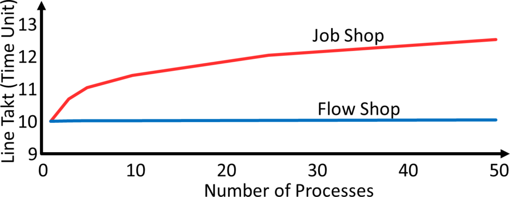
Overall, the flow shop is able to produce goods at a faster rate than the job shop. In fact, for the flow shop the number of processes made only a marginal difference, and the increase in the takt and the decrease in utilization is extremely small. Of course, in reality your system may not behave as nicely as our simulation, but even then I am confident that a flow shop will perform better than a similar job shop.
Inventory and Lead Time
We also looked at the inventory in the system and the closely related lead time for a part to pass through the system. Here, too, the flow shop performed much better. The graphs below show the total inventory in the system for different number of processes. To make the flow shop and the job shop as comparable as possible, we used identical buffer sizes. These buffers decouple fluctuations from the processes (for flow shops and job shops) and differences in the process sequence 8 (for job shops only).
However, the first buffer in the flow shop does not bring any benefit for the system. Since we have an unlimited supply, the first buffer in the flow shop will always be full. Removing the buffer would reduce the inventory by 10 pieces and similarly reduce the lead time. To show a full picture the graph below shows the inventory in the flow shop both with and without the first buffer. if you include the first buffer, the flow shop inventory is always 10 pieces larger.

Based on the inventory and the takt time, we can use Little’s law to calculate the lead time. This is shown below. Similarly to the inventory, we display the flow shop both with and without the first buffer. Since the first buffer always has 10 parts, the difference will always be exactly 10 takt times.

The inventory and the lead time are much better for the flow shop than the job shop. If we exclude the first buffer, both the lead time and the inventory of the flow shop are roughly half that of the job shop. This is a significant difference. You can reduce your lead time by half if you switch from a job shop to a flow shop (at least in theory)!
Other Effects
 Again, I tried to keep the systems as similar as possible. This is also based only on a computer simulation. In reality, you will have more differences. Some of these effects will reduce the difference between flow shops and job shops. For example, your routing may not be as perfectly random as in this simulation. Other effects, however, will make the job shop even worse than the flow shop. For example, a job shop is almost always more difficult to understand and to manage, and in reality you may have to search for parts for the job or search for jobs for the workers. There will be much more friction and mistakes, and hence losses just in knowing what to do where and when. A flow shop will have much fewer problems of this type. See my post on Why Are Job Shops Always Such a Chaotic Mess? for a longer rant about job shops. But overall, I hope that I motivated you toward using flow shops. Now, go out, turn your job shop into a flow shop to gain gargantuan benefits, and organize your Industry!
Source
Daniel Ballach; “Simulation und Gegenüberstellung verrichtungs- und flussorientierter Fertigungssysteme“; Bachelor Thesis, Karlsruhe University of Applied Science, January 1st 2021.
All good stuff …but there’s another means of comparison too. Some year ago I was talking to someone in the broad area of manufacturing air conditioning equipment. I told him of the wonders I’d seen on one of those ‘Cooks Tours’ / ‘Study Tours’ of Japanese Industry, particularly Daikin, which was in the same business. He then told me how much profit they were making …and how much more he was making. Yes, there was the opportunity for him to make a lot more, but he was not too worried!
Hello Steve, Good point. Change usually comes only with pressure. If everybody is comfortable, then why should they change.
Hello Christoph,
Can you tell us the name of the software that was used for those simulations.
Thank you.
Same questions as Jean-Pierre. I would love to know more about the modelling template.
Hello Jean and Jan, the software I used for these simulations is Simul8.
I can recommend Daikin to study something (not only production but management).