
 Having a product mix with different workloads at different stations is challenging. Hence this is getting to be a pretty long series of blog posts on Mixed Model Sequencing. Let’s continue:
Get the Quantities to Be Produced
The next step is a smaller one. You need to figure out the quantities that have to be produced of the different products. The time frame in question is the time frame for which the sequence should hold. Since you don’t known the future, this will be an estimate. As such, it will be flawed. Such is life. Just take the best guess you can and move forward with that number.
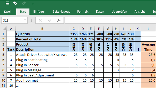
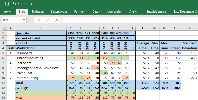
For the Excel example from the last post I added two rows that have the (expected) quantity, for which I also calculated the percentage thereof. Our high runner is model 2437, and our rare exotic models are 2435 and 2440.

Please note that this quantity is the quantity you want to produce in the period you are sequencing. This depends on the cycle time. If it is a fast cycle time (e.g. less than three minutes), you may sequence only for one shift, and create a new sequence again for the next shift. If you have longer cycle times but below an hour you may sequence a day or a week. If your cycle time exceeds hours you may sequence a month. If your cycle time is multiple hours … then you probably don’t need to sequence at all but adjust the capacity by adding or removing workers for one shift to manage the excess workload or excess idle times.
Determine Average Contribution to Cycle Time
The next step is simple math. We would need to figure out how long each step takes on average. The table above gave us the time for each individual step and product type. We now multiply these times with the percentage share of the product type, and sum this up across all products. This gives us the weighted arithmetic mean of the task time. The result could look like this example below.
You could also calculate the maximum, minimum, spread, and standard deviation of the average task time. However, at this time these details are not yet that useful.
Group into Workstation-Sized Workloads
Now comes a more challenging task. You need to group these tasks into groups with the workload for different stations. For now we ignore the times for the individual products and consider only the weighted average time across all products. The total average cycle time across the tasks for one station should be close to the target cycle time (or the average takt time should be close to the target line takt, whichever way you prefer it). If you are a tiny bit above or below the target cycle time, don’t sweat it.
Also keep in mind that you usually can change the sequence somewhat. If I plug in the seat sensor first or the heating first probably does not matter, but it may help you to get a nice average workload for a station. Just make sure the sequence is possible, and that this sequence does not create other problems (i.e., if the worker has to walk from one end of the car to the other end and back).
At the end, all tasks have to be assigned to a workstation, and all workstations have cycle times matching the target cycle time. (If at the end there is work for half a workstation left, try not to spread this time across all workstations, but instead pool it into one workstation. This makes it easier with some improvements to eliminate the workstation altogether for a more efficient line.)
I have written a series of blog posts on this too. Line Balancing Part 5 – Balancing Using Paper and Line Balancing Part 6 – Tips and Tricks for Balancing are the two parts that are most relevant here.
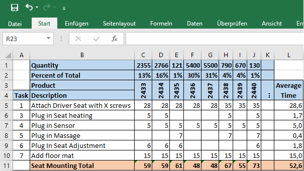
Below would be the example of the seat mounting workstation. The cycle time ranges from 48 seconds (for product numbers 2436 and 2437) to 73 seconds (for product number 2440), with a weighted average of 52.6 seconds. Emphasis on weighted average, as this is not just the average of the individual product times but has to be combined with the percentage of this particular product.
Determine Spread of Workload
Finally you end up with a list of all workstations, how long each product variant takes at each station, and how long it will be in average based on the quantities.
Now we look at the spread of the workloads. You already have the average time for each station. Next we calculate the longest time at each station (i.e., how long does the model with the longest time take at this station). For the dashboard mounting station below, this would be products 2435 and 2440 with 70 seconds cycle time each.
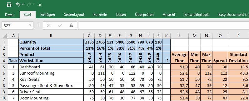
We do the same with the shortest cycle time. For the dashboard station this would be product 2436 and 2439 with 40 seconds each. We also calculate the spread (i.e., the difference between the cycle time of the fastest product and the cycle time of the slowest product). For the dashboard this would be a spread of 30 seconds between the fastest and the slowest product variant. The larger the spread, the more challenging it will be to fit into the average cycle time.
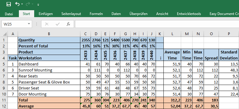
Another value I find useful is the total and average work per product type rather than per workstation. This is shown in the example below. Here product 2437 sticks out with a total workload of 406 seconds total or 67.7 in average, almost twice that of the station with the smallest workload for product 2436 with 37.2 seconds.
Yet another way to analyze the problem is to look a the largest and smallest cycle times for each product. In the example below, I marked the largest and smallest cycle time for each product, with product 2437 and 2434 having the largest cycle times at the sunroof mounting. All other products have the smallest cycle times at the sunroof mounting of zero.
Focus on Your Biggest Rocks first
 Now we have our data together. But before we start sequencing, we have to consider which parts to sequence first. For a good sequencing, we have to start “with the big rocks.” But what do we mean by big? There are many different aspects that come into play:
- Longest Cycle Times: The longer the cycle time, the bigger the problem to fit it into our sequence. Hence, products that have an excessively long cycle time are probably among the first to be sequenced. In our example, products 2437 and 2434 with a sunroof mounting cycle time of 112 and 111 seconds are the largest rocks we have. This is followed by different door mountings, the rear seats, and the dashboard.
- Shortest Cycle Times: These are also relevant, as they may cause excess idle time. They can also be used to counteract the longest cycle times.
- Largest Spread: The difference between the largest cycle time and the shortest cycle time for a station is also relevant, although this is often similar to the parts with the longest and shortest cycle times.
- Largest Average Work per Product: Another way to view this is by looking at the largest average work per product.
- Smallest Average Work per Product: The smallest average work per product can be relevant, similar to the shortest cycle times .
- Largest Cycle Time per Product: And yet another item to consider is the largest cycle time per product
- Smallest Cycle time per Product: Similarly, the smallest cycle time per product may also be relevant to offset the largest ones.
- Largest Quantities Produced: Starting the sequencing with the largest quantity products will help to spread most of the material evenly. If there is no product-dependent workload, then this is the standard approach for sequencing.
Now you have a lot of options for where to start. Unfortunately, a lot of these may be giving you different priorities. A product that has a longest cycle time may also have the shortest at another station, or a perfectly average one at the third. As a small suggestion, you probably can ignore anything that falls within 10% or maybe even 20% of the mean. These will sort itself out by people automatically working a tick faster or slower depending on what is needed.
In the next post I will show you how to make a sequence out of this mess of somewhat conflicting priorities. However, this is not foolproof, and you will need lots of iterations to get to a good solution. Until then, go out, ponder your largest fluctuation, and organize your industry!
P.S. Many thanks to Mark Warren for his input.
Series Overview
- Mixed Model Sequencing – Introduction
- Mixed Model Sequencing – Just Make the Problem Go Away
- Mixed Model Sequencing – Adjust Capacity
- Mixed Model Sequencing – Basic Example Introduction
- Mixed Model Sequencing – Basic Example Workload and Buffering
- Mixed Model Sequencing – Basic Example Sequencing
- Mixed Model Sequencing – Complex Example Introduction
- Mixed Model Sequencing – Complex Example Data Basis
- Mixed Model Sequencing – Complex Example Sequencing 1
- Mixed Model Sequencing – Complex Example Sequencing 2
- Mixed Model Sequencing – Complex Example Verification
- Mixed Model Sequencing – Summary
Here is also the Sequencing Example Excel File for posts 7 to 11 with the complex example. Please note that this is not a tool, but merely some of my calculations for your information.
How can we get a copy of the excel file? I tried to download it but it is pictures.
Hi Alberto, the excel file is quite messy and not cleaned up at all. Hence I prefer not to have it online. For your help, however, I sent you the file as is.
Hi Christoph
I would like a copy of teh excel file Thx.
Hi Alen, I added the excel file for download at the bottom of the post “Series Overview” section.
i would like A EXCEL COPY OF THIS FILE
The link is a the bottom of the post.